Transport of Polystyrene Polymer with DC Motor Having Rollers

Nandigana Venkata Raghavendra Vishal

doi:doi:10.11648/j.eas.20261102.11

Research Article |

| Peer-Reviewed

Transport of Polystyrene Polymer with DC Motor Having Rollers

Nandigana Venkata Raghavendra Vishal^*

Published in Engineering and Applied Sciences (Volume 11, Issue 2)

Received: 16 February 2026 Accepted: 9 March 2026 Published: 19 March 2026

Views: Downloads:

Download PDF

Share This Article

Twitter
Linked In
Facebook

Abstract

In this paper, we study the transport of polystyrene polymer. They are transported using non contact method. We use DC motor having rollers. The motor is connected to switched mode power supply (SMPS) and controller. The voltage of the SMPS is 12 V. The controller controls the voltage of the motor. We study voltage of the motor from 1 V to 8 V. The motor have capacity of 12 V. The current of the motor at 12 V are 1.2 A. The switched mode power supply have electrical plug. We supply 220 V AC supply to SMPS. They have AC to DC converter. Here, the length of the polystyrene is 2 cm, width 2 cm and thickness is 0.082 mm. The mass is measured. We observe the polystyrene do not move from 1 V to 4 V. The transport is from 0.2 cm to 3 cm under the application of 5 V to 8 V, respectively. Further movement are not observed. The multimeters are used to measure the current-voltage characteristics of the motor. They are used to measure the voltage of the SMPS. In this paper, we develop theory to understand the transport of polystyrene under the action of DC motor. We develop two neural network models. The data driven neural network and physics from theory informed in the neural network. The neural network model match the experiments. The accuracy is good. Our simulations use less computer power and time. The training time is 30 s and predict time is 0.07 s. Our work can find applications in printing, packaging, decor, energy, sensors and material handling industries.

Published in	Engineering and Applied Sciences (Volume 11, Issue 2)
DOI	10.11648/j.eas.20261102.11
Page(s)	48-64
Creative Commons	This is an Open Access article, distributed under the terms of the Creative Commons Attribution 4.0 International License (http://creativecommons.org/licenses/by/4.0/), which permits unrestricted use, distribution and reproduction in any medium or format, provided the original work is properly cited.
Copyright	Copyright © The Author(s), 2026. Published by Science Publishing Group

Keywords

DC Motor, Polystyrene, Neural Network, Non-contact Transport, Mass Balance

1. Introduction

The molecular details in the polymers have led to the study and understanding of the structure of polymers. The transport is studied in them

[1-5]

. Polymers are insulating materials. The study of polymers evolved to incorporate the valence, electrons and ions

[6, 7]

. Here, we study polystyrene. They are thermoplastics. Polystyrene have carbon, oxygen and traces of calcium

[8]

. The composition of the elements are obtained from energy dispersive spectroscopy. Polystyrene is thermally stable below 200^◦C. Researchers have studied polystyrene from the ethylene and benzene hybridization fabrication methods

[9]

. The detection of polystyrene with liquid are studied

[10, 11]

. There are needs to relate the concave, convex, bend and chain motion of polystyrene polymer.

Recent studies are available towards aerodynamic drag, speed generated from electric machines and turbines

[12]

. The drag is severe constraint to the efficiency and utilization of energy. The study of drag is critical to transportation and energy applications. The relation between the angular velocity of the electric machine, density of air on the coefficient of aerodynamic drag are studied in detail

[13]

. The conversion of energy from the source to the surface of material is studied using the drag coefficient considering the exposed surface area of the material and drag force. The weight of the material is needed. The friction effects are important

[14]

. The kinetic energy of the air projectiles are often impacted by the surface effects of the material. The source of inlet energy on aerodynamic drag is different from pipe flow

[15]

. Turbulence flow and Reynolds number are the same principles in understanding the drag behavior on surfaces and pipe flow. The knowledge of the drag from the parametric measurement are imperative for economic and environment benefits. The aerodynamic drag lumped effect can be considered wind energy. The correlation of wind from sources are new towards advanced sensor network for migration of energy towards transport

[16]

. The exact mechanical driven system are scope for these studies.

Machine learning (ML) of polymers are studied. The ML methods are used to discover new materials in the polymers

[17-21]

. The availability of data and experiments for polymers are limited. The study of polymers are taken from the membranes, packaging and 3D printing. ML methods gives the details of the polymer using Random Forest Regression, Extreme Gradient Boost, Support Vector Regression (SVR). The clustering of polymers and their properties are studied. The pipeline using ML methods for polymers are well studied

[22, 23]

. The study of deep learning neural network algorithms for polymers are limited. There are studies on metal-ion in polymer matrix. The transport of polymers are studied

[24]

. Over the years the transport of polymers using harvesting methods are considered

[25]

. The structure of polymers, properties and simulation formula are studied

[26-28]

In this paper, we study the transport of polystyrene. We drive the polystyrene using DC motor having rollers. The motor is connected to switched mode power supply, controller and switch. The device is mounted on acrylic slab. The switched mode power supply is connected to electrical plug. We use multimeters to measure the voltage and current of the motor. We develop neural network model to study the transport of polystyrene for the first time. The model matches the experiments. The accuracy is good. Figure 1 shows the schematic of the transport of polystyrene. The length of the polystyrene is 2 cm, width 2 cm and thickness 0.082 mm. They are measured using micrometer. The volume of the polystyrene is

3.28 \times 10^{- 8}

m³. The study of transport of the multiple polystyrenes are the scope for the future work.

The rest of the paper is outlined as follows. Section 2 discusses the materials and methods. Section 3 provides the experiment details. The theory for the polymer transport are given in Section 4. The neural networks simulations that include the data driven neural network and physics from theory in the neural network are given in section 5. A detailed discussion is provided in section 6. Finally, conclusions are presented in Section 7.

2. Materials and Methods

Here, we purchase the polystyrene from Lakshmi electricals and Hardware, India. We use cutter to cut the polystyrene to required size. We purchase cutter from Nimibind, India. We study the size of the polystyrene using plastic scale, vernier caliper and micrometer. The micrometer resolution is 1

μm

. The micrometer, vernier caliper and plastic scale are purchased from Progressive Trade, India. We purchase OM camera. It has microscopy imaging. The OM camera is purchased from Kesari Scientific Chemicals, India. We measure the mass using Kern mass balance. The mass balance accuracy is 0.01 g. They can measure maximum 1200 grams. The mass balance is purchased from Merck, Germany. The switched mode power supply is purchased from Velonix, India. The controller, DC motor having rollers are purchased from Velonix. India. The acrylic base unit to mount the SMPS, controller and DC motor having rollers are fabricated from IITM facility. The electrical wirings are connected. The multimeter port terminals are provided on the acrylic base unit using fabrication facility at IITM. The electrical wirings are connected to the digital multimeters. The multimeters are purchased from electronics, India. The multimeter measures the voltage of the SMPS, voltage of the controller, voltage and the current of the DC motor having rollers. We use four multimeters. The acrylic shield to cover the mass balance are fabricated from IITM facility.

Figure 2 shows the experiment set up. The device consists of switched mode power supply. SMPS have 12 V DC power supply. They have electrical plug of 220 V AC supply. SMPS have AC to DC converter. The other components of the device unit are controller as shown in the Figure 2. The SMPS and controllers are connected to the DC motor having rollers. The acrylic slab is used to mount the devices. The multimeters are connected to the SMPS, controller and DC motor having rollers. The multimeters are plugged to the terminals mounted on the acrylic slab. There are chart paper and book stand as shown in the Figure 2. There are paper tray next to the DC motor having rollers. The polystyrene is placed on the paper tray. The DC motor having rollers are not in contact with the polystyrene. The polystyrene is vertical 2 cm height downward from the black rotating rod of the motor.

Table 1 shows the equipments used in the study. We have switched mode power supply, controller, DC motor having rollers, acrylic slab to mount the devices. The multimeter terminals are placed on the acrylic slab. We use four multimeters. The multimeters are used to measure the voltage and current, respectively. The electrical wirings are available. The chart papers are available on the acrylic slab. The book table of the same height as the acrylic are available next to the acrylic slab. The book table purpose is to show the next region. The polystyrene polymer material is used to study the transport by external DC motor having rollers. The polystyrene is placed on the array of papers. We study non-contact transport of the polystyrene.

Table 2 shows the controller with the knob. The knob on turning gives the desired voltage on the motor. Table 3 shows the parameters of the DC motor having rollers. The diameter of the motor is 26 mm. The shaft diameter that is the roller diameter is 2.3 mm. The shaft is cylinder shape having length 12 mm. The total body length of the DC motor having rollers are 5.7 cm. The maximum voltage of the DC motor is 12 V. The current at 12 V is 1.2 A. The controller controls the voltage of the motor from 0 V to 12 V.

Download: Download full-size image

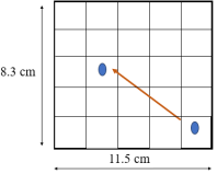
Figure 1. Schematic representation of transport of the polystyrene.

Download: Download full-size image

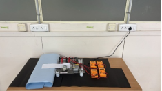
Figure 2. Experiment set up.

Table 1. Equipment list to study the single polystyrene dynamics.

Equipments	Specification details
switched mode power supply (SMPS)	12V
Controller	0 to 12 V controller using knob turns. Also read Table 2
DC motor having rollers	see Table 3
acrylic base
electrical wirings
terminals for the voltage measurement of the SMPS	multimeter wiring plugged for this purpose
terminals for the voltage measurement of the controller	multimeter wiring plugged for this purpose
terminals for the voltage measurement of the DC motor having rollers	multimeter wiring plugged for this purpose
terminals for the current measurement of the DC motor having rollers	multimeter wiring plugged for this purpose
All terminals are placed on the acrylic base. Electrical wirings are available
chart papers are placed on the acrylic table	Many
books are placed next to the acrylic device unit to match the height.	three books
polystyrene is placed on the array of papers	see Table 4 for the dimensions of the polystyrene

Table 2. The relation between the controller knob turns and the voltage.

knob turns in the controller	voltage of the motor (V)
3	1
4	2
5	3
6	4
7	5
8	6
9	7
10	8

Table 3. Parameters of the DC motor having rollers.

Voltage	12V DC
Diameter	26 mm
Speed	18000 rpm
Shaft type	Round type
Shaft length	12 mm
Shaft Diameter	2.3 mm
Total body length	5.7 cm
Current	1.2 A

3. Experiment Details

Table 4 shows the dimensions of the polystyrene. We study polystyrene of length 2 cm, width 2 cm and thickness 0.082 mm. We use plastic scale to measure the length and width of the polystyrene. We use digital micrometer and vernier caliper to measure the thickness of the polystyrene. The volume of the polystyrene is 3.28 × 10^-8m³. Table 4 shows the image of the single polystyrene. The image is taken using OM camera system. Table 4 shows the computer aided design model of the polystyrene. They are modeled using python. Table 5 shows the experiment set up to measure the mass of the polystyrene. We use mass balance. The acrylic shield is used to protect the mass balance. The polystyrene is measured in the box owing to its small mass. The acrylic shield blocks the stream flow to provide steady mass measurement of the polystyrene for the first time. Table 5 shows the dimensions of the polystyrene. We did four repeats to measure the steady mass of the polystyrene as shown in Table 6.

Table 4. Polystyrene geometry, CAD model and image.

Experiment	CAD model	Geometry
		L = 2 cm, B= 2 cm and H = 0.082 mm V = $3.28 \times 10^{- 8}$ m³

Table 5. Mass balance set up. The mass balance is covered with acrylic shield.

Mass measurement set up	Size
	L = 2 cm, B= 2 cm, H = 0.082 mm and V = $3.28 \times 10^{- 8}$ m³

Table 6. Mass of the polystyrene for 4 repeats.

Polystyrene	Trial 1 (mg)	Trial 2 (mg)	Trial 3 (mg)	Trial 4 (mg)
	40	50	34	40

Tables 7-10 shows the device measurements and the maximum distance of the polystyrene. The tables show trial 1, trial 2, trial 3 and trial 4 experiments. We did four repeats. The time is taken in two ways. First, the time is taken when the polystyrene travels the maximum distance. The maximum distance is the final position of the polystyrene. We have observed the polystyrene do not move further this time. Trial 4 are the measurements using the said approach. The second approach is kept simple. The time is recorded when the polystyrene reaches the maximum distance and we wait for some seconds more to ensure there is no further movement of the polystyrene. Trail 1 to Trial 3 readings use the second method. In both methods, the time is recorded using stop watch. The precision of the stop watch is 0.01 s. The distance is measured using micrometer. The resolution of the micrometer is 1 μm.

Table 7. Device measurements and maximum distance of the polystyrene. We show Trial 1 results.

voltage of the DC motor having rollers (V)	current (A)	power (W)	time (s)	distance (m)
1	0.64	0.64	30	0
2	0.71	1.42	30	0
3	0.76	2.28	30	0
4	0.82	3.28	30	0
5	0.85	4.25	7	0.2e-2
6	0.89	5.34	27	1e-2
7	0.92	6.44	16	2e-2
8	1.04	8.32	5	3e-2

Table 8. Device measurements and maximum distance of the polystyrene. We show Trial 2 results.

voltage (V)	current (A)	power (W)	time (s)	distance (m)
1	0.65	0.65	20	0
2	0.72	1.44	20	0
3	0.77	2.31	20	0
4	0.83	3.32	20	0
5	0.87	4.35	17	0.2e-2
6	0.93	5.58	32	1.2e-2
7	0.96	6.72	16	2e-2
8	1.08	8.64	8	3.1e-2

Table 9. Device measurements and maximum distance of the polystyrene. We show Trial 3 results.

voltage (V)	current (A)	power (W)	time (s)	distance (m)
1	0.64	0.64	40	0
2	0.71	1.42	60	0
3	0.78	2.34	60	0
4	0.81	3.24	60	0
5	0.88	4.4	26	0.1e-2
6	0.94	5.64	42	1e-2
7	1.03	7.21	20	2.3e-2
8	1.12	8.96	7	3e-2

Table 10. Device measurements and maximum distance of the polystyrene. We show Trial 4 results.

voltage (V)	current (A)	power (W)	time (s)	distance (m)
1	0.64	0.64	15	0
2	0.72	1.44	16	0
3	0.78	2.34	35	0
4	0.82	3.28	35	0
5	0.86	4.3	7	0.2e-2
6	0.92	5.52	24	1e-2
7	1	7	12	2.1e-2
8	1.14	9.12	5	3e-2

4. Theory

Figure 3(a) shows the schematic understanding of the relation from the power of the motor to the displacement of the polystyrene. Figure 3(b) shows the circuit representation for the transport of the polystyrene with the DC motor having rollers. We study non-contact method of polystyrene transport.

Download: Download full-size image

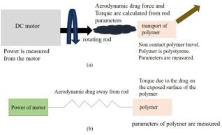
Figure 3. (a) Schematic understanding of the power of the DC motor to displacement of polystyrene polymer (b) Circuit representation of the power of the motor, aerodynamic drag away from the rod and displacement of the polystyrene polymer.

Armature current

We assume the armature shaft current and load current in the DC motor are equal. The armature current is calculated from Eq. (1).

I_{a} = \frac{P}{V}

(1)

where

I_{a}

is the armature current, P is the power and V is the voltage of the DC motor.

Armature Resistance

In this study we use the voltmeter-ammeter method. We lock the motor shaft to prevent rotation. We apply low voltage of 0.2 V to understand the DC motor having rollers do not rotate. The current is 0.61 A. The current is the armature current for the given 0.2 V. The armature resistance is calculated from Eq. (2).

R_{A} = \frac{V}{I_{A}}

(2)

where

R_{A}

is the constant armature resistance for the DC voltage of 0.2 V and corresponding armature current

I_{A}

. Table 11 shows the low DC motor voltage and the corresponding armature current. The constant armature resistance is 0.32 ohm as shown in Table 11.

Table 11. DC voltage, armature current and armature resistance. The motor shaft do not rotate at the low DC voltage.

Armature voltage = 0.2 V

Armature current = 0.61 A

Armature resistance = 0.32 ohm

Back Electromotive force (EMF)

We use voltage equation method to obtain the back electromotive force. The back electromotive force is the magnetic effect in the DC motor. The back electromotive force is calculated using Eq. (3).

E_{b} = V - I_{a} R_{A}

(3)

where

E_{b}

is the back electromotive force. We obtain the back electromotive force for different applied voltage from 1 V to 8 V. The armature current

(I_{a})

for each applied voltage is obtained from Eq. (1). The power of the DC motor is given. The armature resistance

(R_{A})

is fixed to 0.32 ohm. The armature resistance is obtained as discussed earlier. Table 12 shows the back EMF for different voltage of the DC motor.

Table 12. Parameters of the device.

V (volt)	I_a(A)	Power (W)	R_A (ohm)	E_b (V)	Ke (V/(rad/s))	ω (rad/s)	speed (rpm)	Torque (Nm)
1	0.64	0.64	0.32	0.7952	0.0064	124.25	1187.102	0.004096
2	0.71	1.42	0.32	1.7728	0.0064	277	2646.497	0.004544
3	0.76	2.28	0.32	2.7568	0.0064	430.75	4115.446	0.004864
4	0.82	3.28	0.32	3.7376	0.0064	584	5579.618	0.005248
5	0.85	4.25	0.32	4.728	0.0064	738.75	7058.121	0.00544
6	0.89	5.34	0.32	5.7152	0.0064	893	8531.847	0.005696
7	0.92	6.44	0.32	6.7056	0.0064	1047.75	10010.35	0.005888
8	1.04	8.32	0.32	7.6672	0.0064	1198	11445.86	0.006656

Angular velocity of the DC motor shaft

In this paper the maximum voltage of the DC motor is 12 V. At 12 V, the DC motor armature shaft rotates at 18000 revolutions per minute (rpm). The specification chart provides the rpm of the DC motor at 12 V. The angular velocity is calculated using Eq. (4).

ω = \frac{2 πN}{60}

(4)

where

ω

is the angular velocity of the motor shaft. N is the speed of the shaft in revolutions per minute. Table 13 shows the speed and angular velocity of the shaft at 12 V of the motor.

Table 13. Speed and angular velocity of the shaft. The voltage to the motor is 12 V.

rpm	rad/s
18000	1884.96

Motor back electromotive force constant

The motor back electromotive force constant is calculated using Eq. (5).

K_{e} = \frac{V}{ω}

(5)

where

K_{e}

is the back electromotive force constant.

K_{e}

is an intrinsic physical property of the motor. As discussed earlier we know the speed and angular velocity for applied voltage of 12 V on the DC motor. Using Eq. (5) we obtain the back electromotive force constant of 0.0064 V/(rad/s). The voltage is 12 V and angular velocity is 1884.96 rad/s. The back electromotive force constant

K_{e}

is same for different voltage.

Relation between angular velocity and back electromotive force

The back electromotive force is related to the angular velocity of the motor using Eq. (6).

E_{b} = K_{e} ω

(6)

Here, we use the constant

K_{e} = 0.0064

V/(rad/s) as discussed earlier. Table 12 gives the angular velocity of the motor for different back electromotive force. Eq. (4) is used to obtain the speed of the motor. Table 12 shows the speed of the motor in rpm.

Relation between Torque of the motor and armature current

The torque created by the motor is related to the armature current using Eq. (7).

T = K_{e} I_{a}

(7)

where

T

is the torque of the motor. Table 12 shows the torque for different armature current. The armature current are calculated for voltage from 1 V to 8 V.

Figure 4 shows the speed of the motor given in Table 12. The speed is calculated for voltage of the motor from 1 V to 8 V. The torque is linear with the speed of the motor as shown in Figure 4. The slope is

2 \times 10^{- 7}

and the intercept is 0.0039. The torque of the motor are calculated and given in Table 12. The specification of the DC motor provides the speed of the motor is 18000 rpm at 12 V. The instrument motor are calibrated from the literature

[29, 30]

Download: Download full-size image

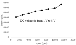
Figure 4. Speed relation with the torque of the motor.

Aerodynamic drag formulation

Table 14 shows the diameter of the motor rotating rod. The diameter of the rod is 3.6 mm. The micrometer is used to measure the diameter of the rod. We measure 4 times the diameter. The trial 1 to trial 4 are given in Table 14.

Table 14. Parameters of the motor rotating rod.

Outer rotating rod of the motor diameter	Trial 1	Trial 2	Trial 3	Trial 4	Instrument used to measure
	3.6 mm	3.6 mm	3.6 mm	3.6 mm	Micrometer

Tangential velocity of the rod of the motor

The tangential velocity of the rod of the motor is calculated using Eq. (8).

v_{t} = r \cdot ω

(8)

where

v_{t}

is the tangential velocity, r is the radius of the rotating rod. The radius of the rod is 0.0018 m. The tangential velocity of the shaft causes the motion of the air. The air offers drag force. The aerodynamic drag are in contact with the polystyrene polymer.

Aerodynamic drag force and drag coefficient

The aerodynamic drag force is calculated using Eq. (9).

F_{d} = μ \cdot w

(9)

where

F_{d}

is the aerodynamic drag force.

μ

is the static friction coefficient. Here

μ = 0.35

for the paper

[31]

. We understand the polystyrene is transported on the array of papers that are kept on the acrylic slab.

w

is the weight of the polystyrene polymer. We consider the mass of the polystyrene is 34 mg in the theory. The weight is calculated using Eq. (10).

w = m \cdot g

(10)

where

m

is the mass of the polystyrene. g is the gravity. The theoretical weight of the polystyrene is

3.34 \times 10^{- 4}

N. Substituting Eq. (10) in Eq. (9) we obtain the aerodynamic drag force. The value is

1.17 \times 10^{- 4}

N. The coefficient of drag is calculated using Eq. (11).

C_{d} = \frac{2 F_{d}}{ρ {\cdot v}_{t}^{2} \cdot A}

(11)

where

C_{d}

is the coefficient of drag.

ρ

is the density of the air. A is the surface area of the polystyrene. The length of the polystyrene is 2 cm. The width is 2 cm and height is 0.082 mm. The volume of the polystyrene is

3.28 \times 10^{- 8}

m³. The surface area of the polystyrene is

4 \times 10^{- 4}

m². Here, we ensure the surface area of the polystyrene are exposed to the air. Table 15 gives the aerodynamic drag parameters. The values are obtained for motor voltage of 8 V.

Table 15. Aerodynamic drag parameters for the motor voltage of 8V.

Density of air	1.225 kg/m³
Surface area of the polystyrene polymer	$4 \times 10^{- 4}$ m²
Angular velocity of motor $ω$	1198 rad/s
Speed of motor	11445.86 rpm
rotating rod diameter	3.6 mm
Tangential velocity $v_{t}$	2.16 m/s
Aerodynamic drag force $F_{d}$	$1.17 \times 10^{- 4}$ N
coefficient of drag $C_{d}$	0.1

Kinematics of the polystyrene Work done by the aerodynamic drag force

The work done by the aerodynamic drag force on the polystyrene is calculated using Eq. (12).

E = \frac{1}{2} m v^{2} + F_{d} \cdot s

(12)

where E is the work done by the aerodynamic drag force.

s

is the displacement of the polystyrene.

v

is the velocity of the polystyrene moving from rest to displacement s.

The velocity of the polystyrene is calculated using Eq. (13).

v = \frac{s}{t}

(13)

where t is the time. Here, we used time given in Table 7. They show trial 1 results. The kinetic energy of the polystyrene is calculated using Eq. (14).

W_{KE} = \frac{1}{2} m v^{2}

(14)

where

W_{KE}

is the kinetic energy of the polystyrene. The aerodynamic drag work is calculated using Eq. (15).

W_{d} = F_{d} \cdot s

(15)

where

W_{d}

is the aerodynamic drag work. The output energy is calculated using Eq. (16).

E = W_{KE} + W_{d}

(16)

where

E

is the output energy. The input electrical energy of the motor is calculated using Eq. (17).

E_{elec} = P \cdot t

(17)

where

E_{elec}

is the input electrical energy of the motor. P is the power of the motor. The power of the motor is calculated using Eq. (18).

P = I_{a} V

(18)

Substituting Eq. (18) to Eq. (17) we obtain the input energy of the motor as given in Eq. (19).

E_{elec} = I_{a} V \cdot t

(19)

We assume small fraction of the input electrical energy is converted to useful displacement of the polystyrene. The theory is for non contact conversion of energy from the motor to displace the polystyrene polymer. The efficiency to convert the electrical energy to useful work is calculated using Eq. (20).

η = \frac{E}{E_{elec}} = \frac{output energy}{input energy}

(20)

Displacement of the polystyrene

The displacement of the polystyrene is calculated using Eq. (12) to Eq. (20). We obtain Eq. (21).

{η I}_{a} Vt = [\frac{1}{2} m \frac{s^{2}}{t^{2}} + F_{d} s]

(21)

We solve Eq. (21) to obtain s. For each voltage applied and time t, the displacement s is obtained by root finding for quadratic equation. The displacement s is calculated using Eq. (22).

s = \frac{- F_{d} + \sqrt{F_{d}^{2} + 4 αE}}{2 α}

(22)

where

α

is calculated using Eq. (23).

α = \frac{1}{2} \frac{m}{t^{2}}

(23)

The output energy

E

is calculated using Eq. (24).

E = η I_{a} Vt

(24)

Table 16. Parameters list 1 relate the power of the motor to the aerodynamic drag and displacement of the polystyrene polymer.

P (W)	t (s)	$E_{elec}$ (J)	r (m)	$v_{t}$ (m/s)	m (kg)
0.64	30	19.2	0.0018	0.23	3.4e-5
1.42	30	42.6	0.0018	0.5	3.4e-5
2.28	30	68.4	0.0018	0.78	3.4e-5
3.28	30	98.4	0.0018	1.05	3.4e-5
4.25	7	29.75	0.0018	1.33	3.4e-5
5.34	27	144.18	0.0018	1.61	3.4e-5
6.44	16	103.04	0.0018	1.89	3.4e-5
8.32	5	41.6	0.0018	2.16	3.4e-5

Table 17. Parameters list 2 to relate the power of the motor to the aerodynamic drag and displacement of the polystyrene polymer.

w (N)	$μ$	$F_{d}$ (N)	$C_{d}$	$η$	$W_{KE}$ (J)	$W_{d}$ (J)	E (J)	Theory s (m)	$v$ (m/s)
3.34e-4	0.35	1.17e-4	9.03					0
3.34e-4	0.35	1.17e-4	1.91					0
3.34e-4	0.35	1.17e-4	0.78					0
3.34e-4	0.35	1.17e-4	0.43					0
3.34e-4	0.35	1.17e-4	0.27	8e-9	1.39e-12	2.33e-7	2.33e-7	2e-3	2.86e-4
3.34e-4	0.35	1.17e-4	0.18	8.2e-9	2.33e-12	1.17e-6	1.17e-6	1e-2	3.7e-4
3.34e-4	0.35	1.17e-4	0.13	2.3e-8	2.66e-11	2.33e-6	2.33e-6	2e-2	1.25e-3
3.34e-4	0.35	1.17e-4	0.10	8.6e-8	6.12e-10	3.5e-6	3.5e-6	3e-2	6e-3

Table 18. Comparison between experiment and theory maximum distance of polystyrene for different motor voltage. The voltage are from 1 V to 8 V.

V (volt)	Theory s (m)	experiment (m)
1	0	0
2	0	0
3	0	0
4	0	0
5	2e-3	2e-3
6	1e-2	1e-2
7	2e-2	2e-2
8	3e-2	3e-2

We use MATAB to solve and obtain s. The roots function in MATLAB provides the maximum displacement of the polystyrene. The parameters of the motor, power, time, input energy, radius of rod of the motor, tangential velocity of motor, mass, weight, aerodynamic drag parameters and output energy are given in Table 16 and Table 17, respectively. The calculated efficiency are given in Table 17. The theoretical displacement of the polystyrene for different power are given in Table 17. The velocity from Eq. (13) for different power are given in Table 17. Table 18 shows the comparison between the theory and experiment maximum distance of the polystyrene for different motor voltage. The voltage is from 1 V to 8 V. The theory match experiments.

5. Data Driven Neural Network Architecture

Figure 5 shows the schematic of the data driven neural network. The neural network uses training data. We provide 3 training data sets. The training data are provided as csv files. In each training data set we have ensured the experiment trial 1, trial 2, trial 3 and trial 4 measurements are uploaded in the csv file. The trial 1, trial 2, trial 3 and trial 4 are repeats of our measurements. The three training data are for motor voltage of 5V, 6V and 7V, respectively. The model is used to predict for DC motor voltage of 8 V.

Download: Download full-size image

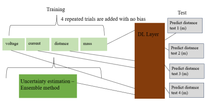
Figure 5. Schematic of Data Driven Neural Network.

Size of Training Data

The training data set 1 have variables [voltage of the motor, current, maximum distance traveled by the polystyrene and mass]. The training data are obtained from experiments. The training data 1 are provided as a csv file. The three training data sets are provided as three csv files, respectively.

Strategy of validation - Uncertainty estimation

Uncertainty estimation provides the confidence to predict the maximum distance traveled by the polystyrene. The confidence is the accuracy of the predict answer to match the experiments. We also measure the mean square error between the predict answer and the actual. This provides the reliable decision-making in AI, engineering, and science. In this paper we use ensemble method to obtain accurate and reliable predict maximum distance of the polystyrene.

Ensemble Method

Here, we provide four trials of our experiment results in the training file. For example, we have three training files. Each file have four variables that are given from measurements. The ensemble method ensures the trial 1, trial 2, trial 3 and trial 4 are in the file. Thus, the training file 1 should have [4× 4] values. The rows are the trial 1, trial 2, trial 3 and trial 4. The column have the discussed [voltage of the motor, current, maximum distance traveled by the polystyrene and mass] variables. The purpose of the ensemble method is discussed in the loss section to obtain the predict maximum distance. The accuracy of the predict distance is highly dependent on the ensemble method.

Control of Fitting – Deep Learning (DL) Layer

We perform the study for 4 voltages. The first three training voltages are 5 V, 6 V and 7V. The fourth voltage is 8 V. The model has to predict the distance for the 8 V. In the first training data file we use control ReLU given in Eq. (25) to obtain the maximum between the two numbers 0 and x₁.

F_{1} = \max (0, x_{1})

(25)

where

F_{1}

is the fit to the variable,

x_{1}

is the distance for voltage of the motor of 5 V. The weight for the first training file are given in Eq. (26) and Eq. (27), respectively.

x_{1} = w_{1} F_{1} + x_{0} + x_{2} + x_{3}

(26)

w_{1} = \frac{x_{1} - x_{0} - x_{2} - x_{3}}{F_{1}}

(27)

where

x_{0}

is the voltage of the motor,

x_{2}

is the current and

x_{3}

is the mass.

w_{1}

is the weight for the training data set 1.

Next, ReLU is done for second training file. Eq. (28) gives the maximum between 0 and

y_{1}

. We denote that as

F_{2}

F_{2} = \max (0, y_{1})

(28)

where

F_{2}

is the fit in the second training set.

y_{1}

is the maximum distance. The weight for the second training file are given in Eq. (29) and Eq. (30), respectively.

y_{1} = w_{2} F_{2} + y_{0} + y_{2} + y_{3}

(29)

w_{2} = \frac{y_{1} - y_{0} - y_{2} - y_{3}}{F_{2}}

(30)

where

y_{0}

is the voltage,

y_{2}

is the current and

y_{3}

is the mass.

w_{2}

is the weight for the training data set 2. We perform the ReLU for third training file. The voltage of the motor under study is 7 V. Eq. (31) gives the maximum between 0 and

z_{1}

. We denote that as

F_{3}

F_{3} = \max (0, z_{1})

(31)

where

F_{3}

is the fit in the third training set.

z_{1}

is the distance in the third training file. The weight for the third training file are given in Eq. (32) and Eq. (33), respectively.

z_{1} = w_{3} F_{3} + z_{0} + z_{2} + z_{3}

(32)

w_{3} = \frac{z_{1} - z_{0} - z_{2} - z_{3}}{F_{3}}

(33)

where

z_{0}

is the voltage,

z_{2}

is the current and

z_{3}

is the mass.

w_{3}

is the weight for the training data set 3. Eq. (27), Eq. (30) and Eq. (33) needs Adam optimizer in python to obtain

w_{1}

w_{2}

w_{3}

and ensuring the loss function in deep learning is compatible with the model in python. The loss function is discussed in the later section.

Linear extrapolation to obtain predict maximum distance for test

We use one data set as test to predict the maximum distance of the polystyrene. The test voltage of the motor is 8 V. Note, the model can predict for any test data set. That is the test data set can be any voltage.

Size of Test Data

The test variables are [voltage, current and mass]. The variables are obtained from experiments. The test file is provided as a csv file. We ensure the trial 1, trial 2, trial 3 and trial 4 measurements for 8 V are in the file. Thus, the test file 1 should have [4× 3] values. The rows are the trial 1, trial 2, trial 3 and trial 4. The column have the discussed [voltage of the motor, current and mass] variables. Remember the column for predict distance are filled with zeroes. We have 4 zeroes in the distance column in the file.

Strategy of validation - Uncertainty Estimation

Here we use ensemble method to ensure the test data set is read correctly. Also, the variables are accurate and reliable to predict the maximum distance.

Ensemble method

The accuracy of the predict distance is highly dependent on the ensemble method. The ensemble of the test file should be detailed as discussed. The loss function are discussed further.

Control of Fitting for Test Data

Here, we use linear extrapolation function in python. The predict maximum distance for test data are given in Eq. (34).

x_{test 1} = w_{1} x_{1} + w_{2} y_{1} + w_{3} z_{1} + x_{test 0} + x_{test 2} + x_{test 3}

(34)

Where

x_{test 1}

is the predict maximum distance for the test data.

x_{test 0}

is the voltage,

x_{test 2}

is the current and

x_{test 3}

is the mass provided in the test file. The weights

w_{1}

w_{2}

and

w_{3}

from the training files are used. The predict maximum distance are obtained for trial 1, trial 2, trial 3 and trial 4. The equation Eq. (34) is put to predict test here. We obtain the predict maximum distance

x_{test 1}

for the trial 1, trial 2, trial 3 and trial 4 properly.

Loss Function

The processor reads the training files. The weight calculations given in Eq. (27), Eq. (30) and Eq. (33) needs the variables as input from the training files. The ensemble method makes sure the variables are fed to calculate the weight. Eq. (34) is done. The ensemble method ensures the task is completed. The loss is minimized in the task. The second loss function is triggered to the display in the model to understand the error between the predict maximum distance and the function Eq. (34) calculation are performable.

Table 19 shows the training file for voltage of the motor of 5 V. The columns are the variables voltage of the motor, current, maximum distance of the polystyrene and mass. The rows are the measured trial 1, trial 2, trial 3 and trial 4 experiment results. Table 20 shows the training file for voltage of the motor of 6 V. Table 21 shows the training file for voltage of the motor of 7 V. Table 22 shows the test file for voltage of the motor of 8 V. The columns are the variables voltage of the motor, current and mass. The column having maximum distance are given 0. They need to be predicted for voltage of the motor of 8 V. The rows are the measured trial 1, trial 2, trial 3 and trial 4 experiment results. Table 23 shows the maximum distance predicted by the data driven neural network for trial 1, trial 2, trial 3 and trial 4 readings. The data driven neural network model matches the experiments. The accuracy is good.

Table 19. Training file 1 having variables [voltage of motor, current, maximum distance of polystyrene and mass] for trial 1, trial 2, trial 3 and trial 4. The trials are given in the rows. The voltage of the motor is 5 V.

V (volt)	current (A)	maximum distance (m)	mass (kg)
5	0.85	2.00E-03	3.40E-05
5	0.87	2.00E-03	4.00E-05
5	0.88	1.00E-03	4.00E-05
5	0.86	2.00E-03	5.00E-05

Table 20. Training file 2 having variables [voltage of motor, current, maximum distance of polystyrene and mass] for trial 1, trial 2, trial 3 and trial 4. The voltage of the motor is 6 V.

V (volt)	current (A)	maximum distance (m)	mass (kg)
6	0.89	1.00E-02	3.40E-05
6	0.93	1.00E-02	4.00E-05
6	0.94	1.00E-02	4.00E-05
6	0.92	1.00E-02	5.00E-05

Table 21. Training file 3 having variables [voltage of motor, current, maximum distance of polystyrene and mass] for trial 1, trial 2, trial 3 and trial 4. The voltage of the motor is 7 V.

V (volt)	current (A)	maximum distance (m)	mass (kg)
7	0.92	2.00E-02	3.40E-05
7	0.96	2.00E-02	4.00E-05
7	1.03	2.30E-02	4.00E-05
7	1	2.10E-02	5.00E-05

Table 22. Test file having variables [voltage of motor, current and mass] for trial 1, trial 2, trial 3 and trial 4. The voltage of the motor is 8 V.

V (volt)	current (A)	mass (kg)
8	1.04	3.40E-05
8	1.08	4.00E-05
8	1.12	4.00E-05
8	1.14	5.00E-05

Table 23. Predict maximum distance of the polystyrene using data driven neural network. The voltage of the motor is 8 V. The rows in the Table imply trial 1, trial 2, trial 3 and trial 4 results.

Predict maximum distance (m)
2.91E-02
2.82E-02
1.93E-02
1.96E-02

Physics Informed Neural Network (PINN)

The only difference between the data driven neural network and the physics informed from theory in the neural network are that in the data driven neural network we provide experiment results as the data. Here in PINN we provide theoretical data. The neural network algorithm remains the same as the data driven neural network. In physics informed from theory in the neural network we have training data and test data. The training variables are voltage of the motor, current, maximum distance of the polystyrene and the mass. The mass of the polystyrene used in the model is 34 mg. We use four repeats instead of trials. Table 24 shows the training file 1. The voltage of the motor is 5 V. Table 25 shows the training file 2. The voltage of the motor is 6 V. Table 26 shows the training file 3. The voltage of the motor is 7 V. The test variables are voltage of the motor, current and the mass of the polystyrene. The mass of the polystyrene used in the model is 34 mg. The column corresponding to the maximum distance are filled with zeroes. Table 27 shows the test file. The voltage is 8 V. Table 28 shows the predict maximum distance of the polystyrene. We obtain for four repeats. The physics from theory in the neural network model matches the experiments. The accuracy is good.

Table 24. Training file 1 in the physics informed from theory in the neural network. The voltage of the motor is 5 V.

V (volt)	current (A)	maximum distance (m)	mass (kg)
5	0.85	2.00E-03	3.40E-05
5	0.85	2.00E-03	3.40E-05
5	0.85	2.00E-03	3.40E-05
5	0.85	2.00E-03	3.40E-05

Table 25. Training file 2. The voltage of the motor is 6 V.

V (volt)	current (A)	maximum distance (m)	mass (kg)
6	0.89	1.00E-02	3.40E-05
6	0.89	1.00E-02	3.40E-05
6	0.89	1.00E-02	3.40E-05
6	0.89	1.00E-02	3.40E-05

Table 26. Training file 3. The voltage of the motor is 7 V.

V (volt)	current (A)	maximum distance (m)	mass (kg)
7	0.92	2.00E-02	3.40E-05
7	0.92	2.00E-02	3.40E-05
7	0.92	2.00E-02	3.40E-05
7	0.92	2.00E-02	3.40E-05

Table 27. Test file for the physics informed from theory in the neural network. The voltage of the motor is 8 V.

V (volt)	current (A)	mass (kg)
8	1.04	3.40E-05
8	1.04	3.40E-05
8	1.04	3.40E-05
8	1.04	3.40E-05

Table 28. Predict maximum distance of the polystyrene using physics informed from theory in the neural network. The voltage of the motor is 8 V.

Predict maximum distance (m)
2.5e-2
2.45e-2
2.45e-2
2.43e-2

6. Results and Discussion

Download: Download full-size image

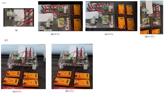
Figure 6. (a-d) Transport for DC = 5 V (a) close picture of polystyrene non contact with the DC motor (b) time, t = 1 s (c) t = 5 s (d) t = 15 s. (e-f) Transport for DC = 8 V (a) move to cm distance observed for polystyrene in non contact drive by DC motor. (e) t = 3 s (f) t = 5 s.

Figure 6(a-d) shows the displacement of the polystyrene at different time. The DC motor have voltage 5 V. Figure 6(e-f) shows the displacement of the polystyrene at different time. The DC motor have voltage 8 V.

Figure 7 shows the comparison of the maximum distance of the polystyrene between the experiment and theory. We study for different power of the DC motor. The theory matches the experiments. The DC motor having rollers are connected to controller and switched mode power supply device. The controller controls the voltage. The DC motor obtains voltage from 1 V to 8 V with the help of the controller. The switched mode power supply have voltage of 12 V.

Download: Download full-size image

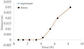
Figure 7. Comparison of the maximum distance of the polystyrene between experiments and theory. The distance is shown for different power of the DC motor.

1) We calculate the residuals (R). The residuals are obtained by calculating the absolute difference between the experiment result and the model. We avoid negative values in the answers because they are physical quantities.

2) We calculate the square of the residuals (R²).

3) The mean square error is calculated. We consider square of the residual.

4) The root mean square error (RMSE) is calculated from the mean square error. We consider the residual as the root mean square error.

Table 29 shows the comparison of the maximum distance of the polystyrene between experiments and data driven neural network. The voltage of the motor is 8 V. We compare between experiment trial 1, trial 2, trial 3 and trial 4 with the data driven neural network results. Table 29 shows the root mean square error. The data driven neural network matches experiments. The accuracy is good. Table 30 shows the comparison of the maximum distance of the polystyrene between the experiments and physics from theory in the neural network. The voltage of the motor is 8 V. We compare between experiment trial 1, trial 2, trial 3 and trial 4 with the physics informed neural network results. Table 30 shows the root mean square error. The physics informed neural network matches experiments. The accuracy is good. In physics from theory in the neural network we tested with 8 repeats for each of the training file. The variables are four. The physics from theory in the neural network model runs and predicts the maximum distance of the polystyrene. They match the experiments. The accuracy is good.

Download: Download full-size image

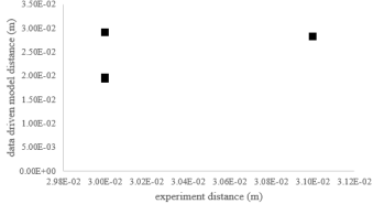
Figure 8. Comparison of the maximum distance of the polystyrene between experiments and data driven neural network. The voltage of the motor is 8 V. We obtain results for different trials.

Download: Download full-size image

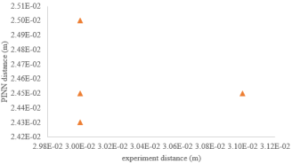
Figure 9. Comparison of the maximum distance of the polystyrene between experiments and physics from theory in the neural network. The voltage of the motor is 8 V. We obtain results for different trials.

Table 29. Comparison of maximum distance of the polystyrene between experiment and data driven neural network. The voltage of the motor is 8 V.

Readings	Experiment maximum distance (m)	Maximum distance from data driven neural network (m)	Residual (R)	(R)²
Trial 1	3e-2	2.91e-2	9e-4	8.1e-7
Trial 2	3.1e-2	2.82e-2	2.8e-3	7.84e-6
Trail 3	3e-2	1.93e-2	1.07e-2	1.14e-4
Trail 4	3e-2	1.96e-2	1.04e-2	1.08e-4

Table 30. Comparison of maximum distance of the polystyrene between experiment and physics from theory in the neural network. The voltage of the motor is 8 V.

Experiment maximum distance (m)	Maximum distance from PINN (m)	Residual (R)	(R)²
3e-2	2.5e-2	5.00E-03	2.50E-05
3.1e-2	2.45e-2	6.50E-03	4.23E-05
3e-2	2.45e-2	5.50E-03	3.03E-05
3e-2	2.43e-2	5.70E-03	3.25E-05

Figure 8 shows the comparison of the maximum distance of the polystyrene between the experiment and data driven neural network. The voltage of the motor is 8 V. The maximum distance of the polystyrene are predicted well. The maximum predict distance for different trials are shown in Figure 8. The model matches experiments. The accuracy of the data driven neural network model is good. Figure 9 shows the comparison of the maximum distance of the polystyrene between the experiments and physics from theory in the neural network. The voltage of the motor is 8 V. The simulation matches experiments. The accuracy of the physics from theory informed in the neural network is good.

7. Conclusions

To conclude, we study the transport the polystyrene polymer using non contact method. We use switched mode power supply, controllers and DC motor having rollers for this purpose. We measure the polystyrene size, volume, mass, current-voltage and power of the motor. We measure the voltage of the switched mode power supply. We develop computer aided design simulation of the polystyrene. We develop neural network models to predict the distance of the polystyrene. The models match the experiments. The accuracy are good. Our work can find applications in sensors, packaging, energy, storage, material handling technology, printing, embossing, automobiles and truck industries.

Abbreviations

SMPS	Switched Mode Power Supply
ML	Machine Learning
SVR	Support Vector Regression
DL	Deep Learning
PINN	Physics Informed Neural Network
RMSE	Root Mean Square Error

Author Contributions

Nandigana Venkata Raghavendra Vishal: Conceptualization, Data curation, Formal analysis, Investigation, Methodology, Resources, Software, Supervision, Validation, Visualization, Writing – original draft, Writing – review & editing.

Data Availability Statement

The data from the current study are available from the corresponding author upon reasonable request.

Conflicts of Interest

The author declares no conflicts of interest.

References

[1]	M. A. Abkowitz, Electronic transport in polymers, Philosophical Magazine B, 65, 817-829, 1992.
[2]	A. Babel, S. A. Jenekhe, High Electron Mobility in Ladder Polymer Field-Effect Transistors, J. Am. Chem. Society, 125, 45, 13656–13657, 2003.
[3]	S. Prodhan, A. Troisi, Effective Model Reduction Scheme for the Electronic Structure of Highly Doped Semiconducting Polymers, J. Chem. Theory Computation, 20, 10147–10157, 2024.
[4]	F. Jeschull, C. Hub et al., Multivalent Cation Transport in Polymer Electrolytes – Reflections on an Old Problem, Advanced Energy Materials, 14, 2302745, 2024.
[5]	H. L. Frisch, C. E. Rogers, Transport in polymers, Journal of Polymer Science Part C: Polymer Symposia, 12, 1966.
[6]	E. Guyon, J. P. Nadal, Y. Pomeau, Disorder and Mixing: Convection, Diffusion and Reaction in Random Materials and Processes, NATO ASI Series E: Applied Sciences, 152, Springer, 1988.
[7]	A. Korolkovas, P. Gutfreund, J. L. Barrat, Simulation of entangled polymer solutions, J. Chem. Phys. 145, 124113, 2016.
[8]	S. Allen, S. D. A. Connell, X. Chen, J. Davies, M. C. Davies, A. C. Dawkes, C. J. Roberts, S. J. B. Tendler, P. M. Williams, Mapping the surface characteristics of polystyrene microtiter wells by a multimode scanning force microscopy approach, Journal of Colloid and Interface Science, 242, 470-476, 2001.
[9]	G. D. Wignall, D. G. H. Ballard, J. Schelten, Chain conformation in molten and solid polystyrene and polyethylene by low-angle neutron scattering, Journal of Macromolecular Science, Part B, 12, 75-98, 1976.
[10]	S. C. Carroccio, P. Cerruti, M. Cervello, A. Cuttitta, P. Colombo, V. Longo, Photoaging of polystyrene-based microplastics amplifies inflammatory response in macrophages, Chemosphere, 364, 1-9, 2024.
[11]	S. Anguissola, D. Garry, A. Salvati, P. J. O Brien, K. A. Dawson, High Content Analysis Provides Mechanistic Insights on the Pathways of Toxicity Induced by Amine-Modified Polystyrene Nanoparticles, Plos One, 9, 1-16, 2014.
[12]	I. Marusic, D. Chandran, A. Rouhi, M. K. Fu, D. Wine, B. Holloway, D. Chung, A. J. Smits, An energy-efficient pathway to turbulent drag reduction, Nature Communications, 12, 1-8, 2021.
[13]	M. P. Ciamarra, A. H. Lara, A. T. Lee, D. I. Goldman, I. Vishik, H. L. Swinney, Dynamics of Drag and Force Distributions for Projectile Impact in a Granular Medium, Phys. Rev. Lett. 92, 194301, 2004.
[14]	M. Di Renzo, J. Urzay, Aerodynamic generation of electric fields in turbulence laden with charged inertial particles, Nature Communications, 9, 1-11, 2018.
[15]	L. Ding, L. F. Sabidussi, B. C. Holloway, A. J. Smits Acceleration is the key to drag reduction in turbulent flow, PNAS, 121, e2403968121, 2024.
[16]	P. Denissenko, S. T. Harvey, An aeroelastic wind energy harvester with continuous orbiting motion and no friction components, Scientific Reports, 15, 34432, 2025.
[17]	T. B. Martin, D. J. Audus, Emerging Trends in Machine Learning: A Polymer Perspective, ACS Polym. Au. 3, 3, 239–258, 2023.
[18]	W. Ge, R. D. Silva, Y. Fan, S. A. Sisson, M. H. Stenzel, Machine Learning in Polymer Research, Advanced Materials, 37, 2413695, 2025.
[19]	R. S. V. D. Hurk, B. W. J. Pirok, T. S. Bos, The role of artificial intelligence and machine learning in polymer characterization: emerging trends and perspectives, Chromatographia, 88, 357–363, 2025.
[20]	D. C. Struble, B. G. Lamb, B. Ma, A prospective on machine learning challenges, progress, and potential in polymer science, MRS Communications, 14, 752–770, 2024.
[21]	B. G. Sumpter, D. W. Noid, Neural networks and graph theory as computational tools for predicting polymer properties, Macromolecular Theory and Simulations, 3, 363-378, 1994.
[22]	P. Reiser, M. Neubert, A. Eberhard, L. Torresi, C. Zhou, C. Shao, H. Metni, C. van Hoesel, H. Schopmans, T. Sommer, P. Friederich, Graph neural networks for materials science and chemistry, Communications Materials, 3, 1-18, 2022.
[23]	T. A. Meyer, C. Ramirez, M. J. Tamasi, A. J. Gormley, A Users Guide to Machine Learning for Polymeric Biomaterials, ACS Polym. Au, 3, 141–157, 2023.
[24]	I. M. Ward, J. Sweeney, Mechanical Properties of Solid Polymers, Third Edition, John Wiley and Sons, Ltd, 2013.
[25]	C. Lodato, F. Magionesi, G. Marsala, A novel energy harvesting technology from the movements of air masses, Discover Applied Sciences, 6, 1-21, 2024.
[26]	J. C. Vidal, J. Midon, A. B. Vidal, D. Ciomaga, F. Laborda, Detection, quantification, and characterization of polystyrene microplastics and adsorbed bisphenol A contaminant using electroanalytical techniques, Microchim Acta, 190, 1-10, 2023.
[27]	A. Motalebizadeh, S. Fardindoost, M. Hoorfar, Selective on-site detection and quantification of polystyrene microplastics in water using fluorescence-tagged peptides and electrochemical impedance spectroscopy, Journal of Hazardous Materials, 480, 136004, 2024.
[28]	C. Mayorga, S. M. Athalye, M. Boodaghidizaji, N. Sarathy, M. Hosseini, A. Ardekani, M. S. Verma, Limit of Detection of Raman Spectroscopy Using Polystyrene Particles from 25 to 1000 nm in Aqueous Suspensions, Anal. Chem., 97, 8908–8914, 2025.
[29]	G. A. Sziki, K. Sarvajcz, J. Kiss, T. Gal, A. Szanto, A. Gabora, G. Husi, Experimental investigation of a series wound DC motor for modeling purpose in electric vehicles and mechatronics systems, Measurement, 109, 111-118, 2017.
[30]	R Morales, J A Somolinos, H S Ramirez, Control of a DC motor using algebraic derivative estimation with real time experiments, Measurement, 47, 401-417, 2014.
[31]	Aerodynamic drag parameters study Available from: https://web.mit.edu/8.13/8.13c/references-fall/aip/aip-handbook-section2d.pdf (accessed 12 January 2026).

Cite This Article

Plain Text BibTeX RIS

APA Style

Vishal, N. V. R. (2026). Transport of Polystyrene Polymer with DC Motor Having Rollers. Engineering and Applied Sciences, 11(2), 48-64. https://doi.org/10.11648/j.eas.20261102.11

Copy | Download

ACS Style

Vishal, N. V. R. Transport of Polystyrene Polymer with DC Motor Having Rollers. Eng. Appl. Sci. 2026, 11(2), 48-64. doi: 10.11648/j.eas.20261102.11

Copy | Download

AMA Style

Vishal NVR. Transport of Polystyrene Polymer with DC Motor Having Rollers. Eng Appl Sci. 2026;11(2):48-64. doi: 10.11648/j.eas.20261102.11

Copy | Download

@article{10.11648/j.eas.20261102.11,
  author = {Nandigana Venkata Raghavendra Vishal},
  title = {Transport of Polystyrene Polymer with DC Motor Having Rollers},
  journal = {Engineering and Applied Sciences},
  volume = {11},
  number = {2},
  pages = {48-64},
  doi = {10.11648/j.eas.20261102.11},
  url = {https://doi.org/10.11648/j.eas.20261102.11},
  eprint = {https://article.sciencepublishinggroup.com/pdf/10.11648.j.eas.20261102.11},
  abstract = {In this paper, we study the transport of polystyrene polymer. They are transported using non contact method. We use DC motor having rollers. The motor is connected to switched mode power supply (SMPS) and controller. The voltage of the SMPS is 12 V. The controller controls the voltage of the motor. We study voltage of the motor from 1 V to 8 V. The motor have capacity of 12 V. The current of the motor at 12 V are 1.2 A. The switched mode power supply have electrical plug. We supply 220 V AC supply to SMPS. They have AC to DC converter. Here, the length of the polystyrene is 2 cm, width 2 cm and thickness is 0.082 mm. The mass is measured. We observe the polystyrene do not move from 1 V to 4 V. The transport is from 0.2 cm to 3 cm under the application of 5 V to 8 V, respectively. Further movement are not observed. The multimeters are used to measure the current-voltage characteristics of the motor. They are used to measure the voltage of the SMPS. In this paper, we develop theory to understand the transport of polystyrene under the action of DC motor. We develop two neural network models. The data driven neural network and physics from theory informed in the neural network. The neural network model match the experiments. The accuracy is good. Our simulations use less computer power and time. The training time is 30 s and predict time is 0.07 s. Our work can find applications in printing, packaging, decor, energy, sensors and material handling industries.},
 year = {2026}
}

Copy | Download

TY - JOUR
T1 - Transport of Polystyrene Polymer with DC Motor Having Rollers
AU - Nandigana Venkata Raghavendra Vishal
Y1 - 2026/03/19
PY - 2026
N1 - https://doi.org/10.11648/j.eas.20261102.11
DO - 10.11648/j.eas.20261102.11
T2 - Engineering and Applied Sciences
JF - Engineering and Applied Sciences
JO - Engineering and Applied Sciences
SP - 48
EP - 64
PB - Science Publishing Group
SN - 2575-1468
UR - https://doi.org/10.11648/j.eas.20261102.11
AB - In this paper, we study the transport of polystyrene polymer. They are transported using non contact method. We use DC motor having rollers. The motor is connected to switched mode power supply (SMPS) and controller. The voltage of the SMPS is 12 V. The controller controls the voltage of the motor. We study voltage of the motor from 1 V to 8 V. The motor have capacity of 12 V. The current of the motor at 12 V are 1.2 A. The switched mode power supply have electrical plug. We supply 220 V AC supply to SMPS. They have AC to DC converter. Here, the length of the polystyrene is 2 cm, width 2 cm and thickness is 0.082 mm. The mass is measured. We observe the polystyrene do not move from 1 V to 4 V. The transport is from 0.2 cm to 3 cm under the application of 5 V to 8 V, respectively. Further movement are not observed. The multimeters are used to measure the current-voltage characteristics of the motor. They are used to measure the voltage of the SMPS. In this paper, we develop theory to understand the transport of polystyrene under the action of DC motor. We develop two neural network models. The data driven neural network and physics from theory informed in the neural network. The neural network model match the experiments. The accuracy is good. Our simulations use less computer power and time. The training time is 30 s and predict time is 0.07 s. Our work can find applications in printing, packaging, decor, energy, sensors and material handling industries.
VL - 11
IS - 2
ER -

Copy | Download

Author Information

Nandigana Venkata Raghavendra Vishal

Department of Mechanical Engineering, Indian Institute of Technology Madras, Chennai, India

Contact Email

http://orcid.org/0009-0000-6260-6567

Download PDF

Submit an Article

Plain Text BibTeX RIS

APA Style

Vishal, N. V. R. (2026). Transport of Polystyrene Polymer with DC Motor Having Rollers. Engineering and Applied Sciences, 11(2), 48-64. https://doi.org/10.11648/j.eas.20261102.11

Copy | Download

ACS Style

Vishal, N. V. R. Transport of Polystyrene Polymer with DC Motor Having Rollers. Eng. Appl. Sci. 2026, 11(2), 48-64. doi: 10.11648/j.eas.20261102.11

Copy | Download

AMA Style

Vishal NVR. Transport of Polystyrene Polymer with DC Motor Having Rollers. Eng Appl Sci. 2026;11(2):48-64. doi: 10.11648/j.eas.20261102.11

Copy | Download

@article{10.11648/j.eas.20261102.11,
  author = {Nandigana Venkata Raghavendra Vishal},
  title = {Transport of Polystyrene Polymer with DC Motor Having Rollers},
  journal = {Engineering and Applied Sciences},
  volume = {11},
  number = {2},
  pages = {48-64},
  doi = {10.11648/j.eas.20261102.11},
  url = {https://doi.org/10.11648/j.eas.20261102.11},
  eprint = {https://article.sciencepublishinggroup.com/pdf/10.11648.j.eas.20261102.11},
  abstract = {In this paper, we study the transport of polystyrene polymer. They are transported using non contact method. We use DC motor having rollers. The motor is connected to switched mode power supply (SMPS) and controller. The voltage of the SMPS is 12 V. The controller controls the voltage of the motor. We study voltage of the motor from 1 V to 8 V. The motor have capacity of 12 V. The current of the motor at 12 V are 1.2 A. The switched mode power supply have electrical plug. We supply 220 V AC supply to SMPS. They have AC to DC converter. Here, the length of the polystyrene is 2 cm, width 2 cm and thickness is 0.082 mm. The mass is measured. We observe the polystyrene do not move from 1 V to 4 V. The transport is from 0.2 cm to 3 cm under the application of 5 V to 8 V, respectively. Further movement are not observed. The multimeters are used to measure the current-voltage characteristics of the motor. They are used to measure the voltage of the SMPS. In this paper, we develop theory to understand the transport of polystyrene under the action of DC motor. We develop two neural network models. The data driven neural network and physics from theory informed in the neural network. The neural network model match the experiments. The accuracy is good. Our simulations use less computer power and time. The training time is 30 s and predict time is 0.07 s. Our work can find applications in printing, packaging, decor, energy, sensors and material handling industries.},
 year = {2026}
}

Copy | Download